stivenmosheyoff/BankChurners

Why Do Some Customers Spend More? - Classification, Regression, Clustering, Evaluation

Author: stiven rodriguez Course: Introduction to Data Science Assignment: Classification, Regression, Clustering, Evaluation Dataset Source: Kaggle – Predicting Credit Card Customer Segmentation Dataset Size: ~10,128 rows × 22 column

Project Goal

The objective of this project is to analyze credit card usage patterns to predict and classify customer spending levels (Low, Medium, or High) . By combining unsupervised clustering for customer profiling with advanced supervised learning models (like Gradient Boosting) , the solution enables the bank to implement precise, data-driven marketing and retention strategies.

Part 1: Exploratory Data Analysis (EDA)

Dataset Overview

• gender - ( male=1 , female=0)
• Education_Level - (Uneducated = 1, High School = 2, College = 3, Graduate = 4, Post-Graduate = 5, Doctorate = 6)
• Attrition_Flag – whether the customer stayed or left (Existing Customer = 1 Attrited Customer = 0
• Customer_Age – how old the customer is
• Marital_Status – whether the customer is married or single
• ('Married' = 1 ,'Single' = 0)
• Income_Category – the customer’s income level
• (Less than $40K = 1 , $40K - $60K = 2 , $60K - $80K = 3 , $80K - $120K , = 4 , $120K + = 5 )
• Card_Category – the type of credit card they have
• (Blue = 1 , Silver = 2 ,Gold = 3 ,Platinum = 4)
• Months_on_book – how many months they have been a customer
• Total_Relationship_Count – how many products the customer has with the bank
• Months_Inactive_12_mon – how many inactive months they had in the last year
• Contacts_Count_12_mon – how many times the customer contacted the bank
• Credit_Limit – the customer’s credit limit
• (0-2.5k) = 0, (2.5k-5k) = 1,(5k-7.5k) = 2,(7.5k-10k) = 3,(10k-12.5k) = 4, (12.5k-17.5k) = 5, (17.5k-30k) = 6, (30k+) =7)
• Total_Revolving_Bal – how much money the customer still owes
• Total_Trans_Amt – total amount of money spent
• Total_Trans_Ct – total number of transactions made
• Avg_Utilization_Ratio – how much of their credit limit they use

The final dataset is the result of systematic cleaning, validation, and filtering procedures

Data Cleaning Summary

• Selected 19 relevant columns from the original 22 columns for analysis.
• Handling Non-Informative
• create new columns
• Removing Duplicates
• Converting Relevant Variables to Numeric Format
• Missing Value Handling, Removing Missing Columns
• Filtering Out NaN income Customer Profiles
• Filtering Out Incomplete Customer Profiles (Less Than 12 Months Tenure)
• Filling Missing 'Stance' Values with 'Unknown
• Converting Relevant Variables to Numeric Format Before Outlier Analysis
• Outlier Detection & Handling

Research Questions & Insights

Key Drivers of Customer Spending

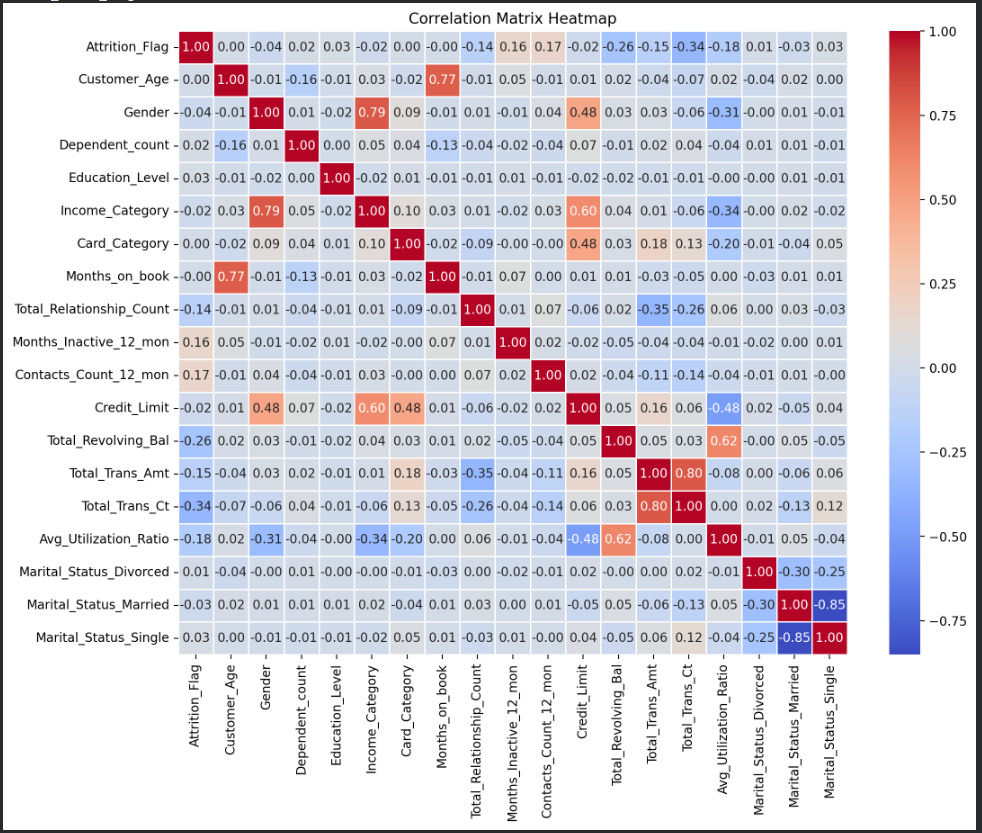
1."Which features show the strongest correlation with the Total Transaction Amount?

Visualization: Correlation Heatmap of Variables Click on the image above to view it in full size Insight:

• My conclusion is that this feature has a negative correlation of –35% with Total_Relationship_Count, meaning it tends to be higher among customers who have fewer products with the bank. This suggests the feature is more common among less engaged or newer customers, which explains the negative relationship. Additionally, the feature shows a positive correlation of 16% with Credit_Limit and 18% with Card_Category, indicating that customers with higher credit limits or higher-tier cards tend to have slightly higher values of this feature.

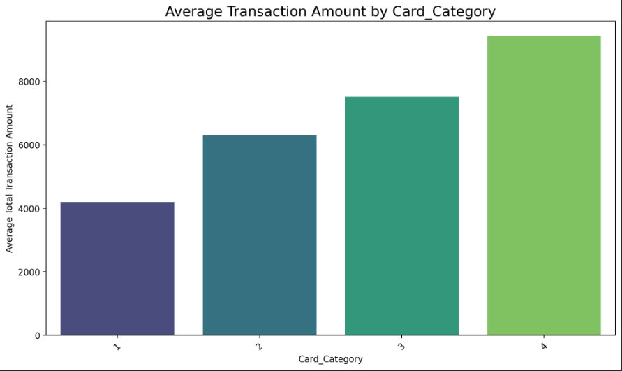
2. What is the impact of the Card Category on the Total Transaction Amount?

Visualization: bar plot Click on the image above to view it in full size Insight:

• My conclusion is that higher card categories are associated with higher customer spending. As the card tier increases, the average total transaction amount consistently rises, indicating that customers with premium cards tend to spend significantly more than those with basic card types.

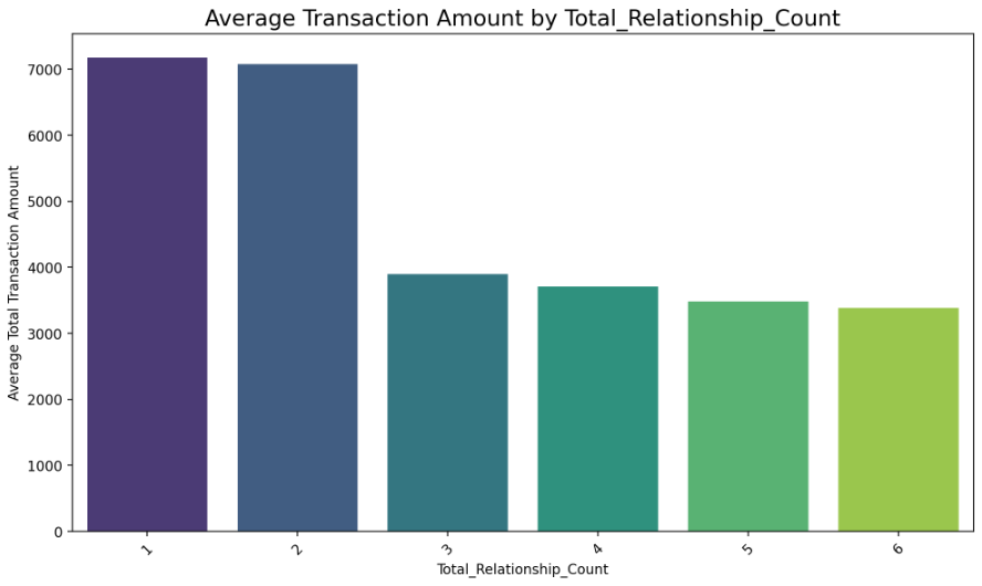
3. What is the impact of the relationships customer has with the credit card provider

on the Total Transaction Amount?

Visualization: bar plot Click on the image above to view it in full size Insight:

• My conclusion is that customers with fewer banking relationships tend to spend more. Those with only 1–2 products show the highest average transaction amounts, while customers with more products (3–6) spend significantly less on average. This indicates a negative relationship between the number of bank products a customer holds and their total spending.

Final Conclusions

Main Research Question: Why Do Some Customers Spend More? Answer: The analysis clearly shows how different customer features are related to Total Transaction Amount (Total_Trans_Amt). By examining correlations and comparing average spending across key variables, we identify several consistent patterns that explain what drives higher or lower transaction amounts among customers. These findings support better customer segmentation and help highlight the factors most strongly associated with spending behavior.

Key Findings:

Key Findings

1. Transaction Activity Drives Spending Total_Trans_Ct is the strongest predictor of Total_Trans_Amt, showing a strong positive correlation. Customers who complete more transactions also spend significantly more.

2. Card Tier Influences Transaction Amount Higher Card_Category levels are associated with higher average transaction amounts. Premium cardholders tend to be more active and spend more overall.

3. Utilization Ratio Reflects Customer Activity Avg_Utilization_Ratio has a moderate positive correlation with spending. Customers who use a larger portion of their credit limit tend to perform more—or larger—transactions.

4. Customer Age and Demographics Have Minimal Impact Variables such as age, gender, and marital status show near-zero correlation with spending. These demographic attributes do not meaningfully influence transaction behavior.

5. Relationship Depth Shows a Reverse Pattern Customers with fewer products (e.g., 1–2 relationships) have higher average transaction amounts. As Total_Relationship_Count increases, spending decreases—indicating a negative relationship. This may reflect that highly engaged customers distribute their financial activity across more products (e.g., savings, loans), reducing their card spending.

6. Secondary Correlations Weak positive correlations with Credit_Limit and Card_Category, and a negative correlation with Total_Relationship_Count, reinforce earlier behavioral insights.

Overall Insights:

Overall Insights

High spenders are not necessarily highly engaged customers. Customers with fewer bank products tend to concentrate their financial activity in card transactions, resulting in higher spending.

Premium cardholders represent a valuable segment. They show consistently higher spending and may serve as ideal targets for personalized offers or loyalty programs.

Transaction frequency is a key behavioral indicator. It explains more variance in spending than any demographic attribute or credit limit measure.

Utilization patterns signal financial activity intensity. Customers with higher utilization ratios may be more responsive to credit limit adjustments or risk assessments.

Segmentation Opportunities: The patterns identified can help define customer groups such as high-spending low-engagement customers, active premium users, or low-risk but low-activity customers.

Part 2: Define and Train a baseline model

• 1. Regression Goal: The goal of this regression is to predict the total transaction amount based on demographic, behavioral, and financial features
• 2. Feature Selection: For the baseline model, all available numerical and encoded categorical features were included, excluding the target variable (Total_Trans_Amt) and the churn indicator (Attrition_Flag). This approach aligns with a baseline strategy where the goal is to establish initial performance before performing feature optimization.
• 3. Train–Test Split: The dataset was split into training and testing sets using an 80/20 ratio
• 4. Model Training: This model serves as a starting benchmark for future comparisons with more advanced models.
• 5. Model Evaluation: MAE ≈ 1395.8 MSE ≈ 3,655,754 RMSE ≈ 1912.0 R² ≈ 0.68 These results indicate that the baseline model explains approximately 68% of the variance in transaction amounts. While reasonably strong for a linear baseline, the model still struggles with customers who have very high spending, suggesting non-linear patterns in customer behavior.
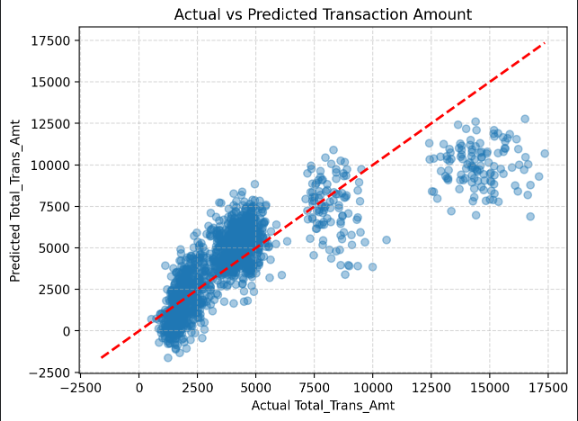
• 6. Insights – Visuals: Click on the image above to view it in full size A scatter plot of actual vs. predicted transaction amounts shows that:The model captures the general trend well. Prediction errors increase at higher spending levels. This behavior is expected from a simple linear model when the underlying relationships may be partially non-linear.
• 7. Feature Importance: 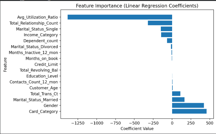Click on the image above to view it in full size

Summary of Baseline Model Insights

The model performs moderately well for a first attempt, achieving an R² of 0.68. Transaction frequency (Total_Trans_Ct) is one of the strongest predictors of spending. Certain behavioral and demographic features also play an important role, while others have minimal impact. This baseline establishes a solid foundation for future model improvements such as polynomial features, regularization, or tree-based models.

Part 3 — Feature Engineering (Summary)

This section focuses on creating new informative features through scaling, transformation, and clustering, as required in the assignment.

Feature Scaling

Selected behavioral and financial variables (Total_Trans_Ct, Total_Revolving_Bal, Avg_Utilization_Ratio, Total_Relationship_Count, Credit_Limit) were standardized using StandardScaler, as required for clustering algorithms.

Clustering Model (Required Feature Engineering Step)

A K-Means model with 4 clusters was trained on the scaled features. Two new features were created as required: Cluster_ID — the cluster assignment for each customer Dist_To_Centroid — distance from each sample to its closest cluster center (measures typicality) Cluster_ID was then one-hot encoded, making the clustering results usable in downstream supervised models.

PCA Visualization

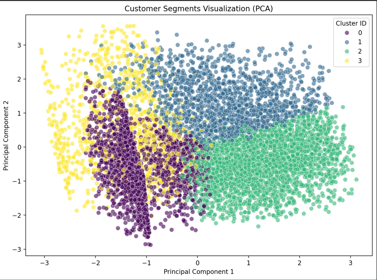PCA was applied to reduce the scaled feature space to 2 components, enabling a clear visualization of the four customer segments and validating the clustering structure.

• Cluster Interpretation Cluster-level mean statistics were computed to profile each customer segment and understand behavioral differences relevant to transaction patterns.

• Outcome All required elements of Part 4 were completed: scaling, feature creation, categorical encoding, clustering-based feature engineering, PCA visualization, and segment interpretation.

Part 4 — Improved Model Training & Evaluation

1. Retrain Linear Regression with Engineered Features

The baseline Linear Regression model was retrained using the full engineered dataset, which includes:

cluster features (Cluster_*, Dist_To_Centroid)

scaled numerical variables

encoded categorical features

This provides a fair, improved benchmark for comparison.

2. Train Two Additional Sklearn Models

Two non-linear models were trained on the same engineered dataset:

Random Forest Regressor

Gradient Boosting Regressor

Both models come from the sklearn library, satisfying the requirement for multiple model types.

3. Compare Performance with Baseline

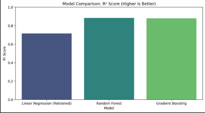Each model was evaluated using: MAE, RMSE, R²

The results clearly show improvement over the baseline and over the retrained Linear Regression model. A bar plot visualized the R² values of all models for easy comparison.

4. Visualize Feature Importance

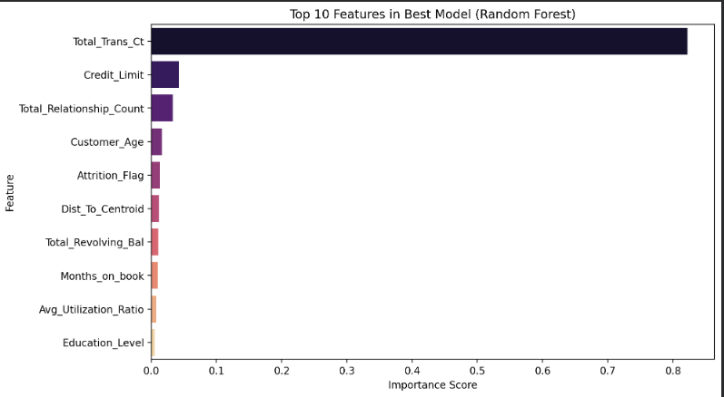For the best-performing model (Random Forest), the top 10 most important features were plotted using feature_importances_. Key drivers include:

Total_Trans_Ct, Credit_Limit, Total_Relationship_Count ,Dist_To_Centroid

This demonstrates how the engineered features impact the final prediction.

5. Discuss Improvement

Model performance improved significantly (+27% vs. baseline). Tree-based models perform better because they:

capture non-linear relationships

learn interactions between variables

leverage the cluster-based features more effectively

6. Declare the Winner

The best model based on R² performance:

🏆 Random Forest Regressor (R² ≈ 0.838)

Part 5: Regression-to-Classification

Part 5.1 — Creating Target Classes

In this step, the original continuous target variable (Total_Trans_Amt) was transformed into discrete categories to reframe the regression problem as a classification task. A quantile-based binning strategy (q=3) was applied, creating three balanced classes:

Class 0 – Low spenders (bottom 33%)

Class 1 – Medium spenders (middle 33%)

Class 2 – High spenders (top 33%)

This approach ensures evenly distributed classes and provides meaningful business segmentation (e.g., retention for low spenders, upselling for medium, and VIP targeting for high spenders). The same engineered features from previous sections were used, and the dataset was properly split into train and test sets without data leakage.

Part 5.2 — Required Answers

• 1️ Show the resulting class distribution (counts or percentages).

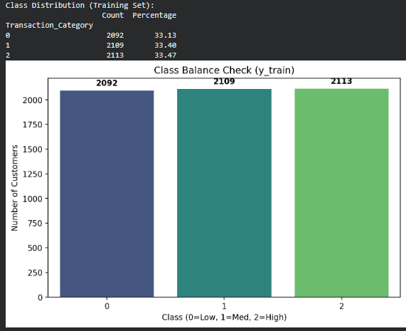
Class 0 = 2,092 (33.13%) Class 1 = 2,109 (33.40%) Class 2 = 2,113 (33.47%)

This indicates equal-sized groups created by the qcut method.

• 2️ Are some classes under-represented? No. All three classes have almost identical proportions (~33% each). Therefore, the dataset is well balanced.

• 3️ If the data is imbalanced, explain which metric you’ll focus on and why accuracy alone is misleading. Since the classes are balanced, using Accuracy as the main evaluation metric is appropriate. (Theory explanation included:) Accuracy becomes misleading only when one class dominates. For example, if 90% of customers were Class 0, a model guessing only Class 0 could score 90% accuracy

while completely failing to detect the other classes. In such cases, F1-score or Recall would be preferred.

• 4️ If needed, consider changing your conversion. No changes were needed. The quantile-based binning (qcut) already produced balanced class groups, so the conversion method is appropriate and remains unchanged.

Part 6 — Classification Modeling (Summary)

6.1 — Precision vs Recall & Error Types

Precision vs Recall In this customer segmentation task, recall for the High spending class is more important than precision. Missing a true high-value customer means failing to offer them VIP benefits or retention incentives, increasing the risk of churn. It is less harmful to mistakenly classify a Medium customer as High than to overlook a true High spender.

False Positives vs False Negatives A False Negative (a true High spender predicted as Medium/Low) is more critical than a False Positive. A False Negative may cause the company to ignore a valuable customer segment, while a False Positive only results in minor overspending on marketing. Therefore, minimizing False Negatives is a priority.

6.2 — Training Three Classification Models

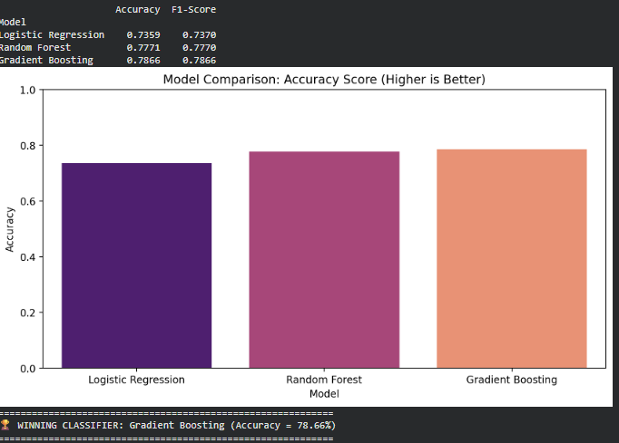
Three different classification models were trained on the engineered feature set: Logistic Regression (linear model) Random Forest Classifier (bagging, tree-based) Gradient Boosting Classifier (boosting, tree-based)

Each model was evaluated using Accuracy and Weighted F1-Score. Results show that tree-based methods outperform the linear baselin

Part 6.3 — Classification Model Evaluation

1. Logistic Regression

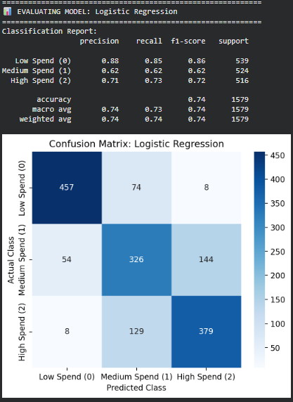
• Performance (Classification Report) Accuracy: 0.74 Strong performance on Low Spend customers Weaker precision/recall for Medium and High spenders (F1 ≈ 0.62–0.73)
• Error Analysis (Confusion Matrix) Significant confusion between Medium (1) and High (2) The model often predicts the “middle” class (Class 1), indicating a tendency to underfit non-linear boundaries.

2. Random Forest Classifier

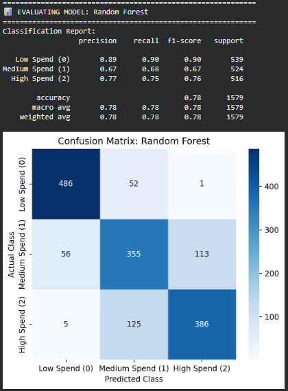
• Performance Accuracy: 0.78 Better balance across classes compared to Logistic Regression Improved F1-scores for Medium and High spenders
• Error Analysis Fewer mistakes overall Still exhibits noticeable confusion between Medium and High spenders, though less severe than Logistic Regression.

3. Gradient Boosting Classifier

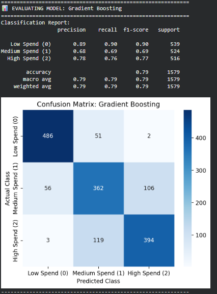
• Performance Accuracy: 0.79 (best overall) Highest F1-scores across all classes Strong performance on the critical High spender group
• Error Analysis Produces the fewest misclassifications across all classes Very low False Negatives for the High spender segment — important for customer retention and targeted marketing Handles class boundaries more effectively than the other models

Best Model: Gradient Boosting Classifier

Gradient Boosting achieved the highest Accuracy and F1-score, and produced the most stable class predictions. It made the fewest critical mistakes — especially avoiding False Negatives for High spenders, which is key from a business perspective. Its ability to capture complex, non-linear relationships makes it the superior model for this classification task.